Modern machine learning systems rely on computational architectures that transform inputs into predictions through layered connections. These structures, often termed deep learning models, adjust their internal parameters using mathematical principles to minimise errors. At the heart of this process lies the concept of gradient optimisation—a method tracing its roots to pioneering work by Rumelhart, Hinton, and Williams in 1986.
Training such systems involves two phases: forward propagation for inference and backward propagation for parameter updates. The latter utilises gradient information to determine precise adjustments, ensuring models improve iteratively. This approach became foundational for architectures like LeNet and AlexNet, revolutionising fields from computer vision to natural language processing.
Understanding these mechanisms requires grasping how layered networks process data. Each layer applies weighted transformations, with errors measured against desired outputs. The critical role of gradients emerges here—they quantify how sensitive the system’s performance is to each parameter. Mastery of this principle enables practitioners to optimise models effectively, bridging theoretical mathematics with real-world applications.
This guide unpacks the mathematical and practical aspects of gradient-based training. Readers will gain insights into both the historical evolution of these techniques and their modern implementations. By the end, you’ll possess the conceptual toolkit needed to work confidently with contemporary deep learning frameworks.
Introduction to Neural Networks and Gradients
Computational systems inspired by biological cognition form the backbone of modern artificial intelligence. These architectures process data through layered nodes, mimicking synaptic connections observed in natural brains. Unlike biological systems, however, they depend on mathematical frameworks to refine their predictive capabilities.
Overview of Neural Network Concepts
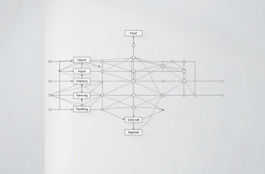
Artificial neurons organise into interconnected layers, transforming inputs via weighted connections. During forward propagation, data flows through these layers to generate outputs. This phase demonstrates the system’s inference capabilities without altering its parameters.
Training occurs through iterative adjustments. Errors between predictions and actual outcomes drive backward propagation. Here, the architecture identifies which connections require modification to improve accuracy.
Importance of Gradients in Model Training
Gradients serve as directional guides for parameter updates. They quantify how each weight influences overall performance, enabling precise adjustments. This mathematical approach eliminates guesswork in optimisation.
By analysing gradient magnitudes, systems prioritise changes with the highest impact. Such targeted learning allows models to uncover complex patterns autonomously. This principle underpins advancements in speech recognition, medical diagnostics, and financial forecasting.
Fundamentals of Calculus in Neural Networks
Mathematical principles from calculus underpin the training processes of modern learning systems. These tools quantify relationships between inputs and outputs, enabling precise adjustments during optimisation. At their core, they measure how minute changes in variables affect overall system performance.

Understanding Derivatives and Slope
A derivative represents the rate change of a function at a specific point. For example, consider f(x) = x² – 16. Its derivative, f'(x) = 2x, reveals how steeply the curve ascends or descends at any x-value. This slope concept extends directly to training scenarios where systems assess error sensitivity.
In single-variable contexts, derivatives provide straightforward directional guidance. They indicate whether increasing or decreasing a parameter reduces errors. This principle becomes foundational when scaling to complex, multi-parameter models.
Role of Partial Derivatives in Multivariable Functions
Real-world systems rarely depend on single inputs. Partial derivatives isolate the impact of individual variables while keeping others constant. For a function like f(x,y) = 3x² + 2y, ∂f/∂x = 6x and ∂f/∂y = 2 measure each input’s unique contribution.
These calculations combine into a gradient vector (∇f), guiding coordinated parameter updates. In layered architectures, this approach ensures weights adjust proportionally to their influence on outcomes. Such precision enables efficient learning across thousands of interconnected nodes.
Understanding Gradient Descent and Its Role in Optimisation
Parameter adjustment techniques form the backbone of modern machine learning. Among these, gradient descent stands out as the most widely used method for navigating complex mathematical landscapes. Its iterative approach balances computational efficiency with practical effectiveness.
Defining Gradient Descent
The descent algorithm operates like a hiker finding the quickest path downhill. Starting from random coordinates, it calculates local slope information using first derivatives. Parameters update repeatedly using the formula:
| Step | Action | Purpose |
|---|---|---|
| 1 | Initialise weights | Establish starting point |
| 2 | Compute gradient | Determine steepest descent |
| 3 | Adjust parameters | Move towards minimum |
| 4 | Check convergence | Evaluate progress |
The learning rate (α) controls step sizes. Too large, and the system overshoots valleys. Too small, and progress becomes glacial. Proper tuning ensures steady movement towards the global minimum.
Comparison With Other Optimisation Methods
Newton-Raphson methods employ second derivatives for precise curvature analysis. While theoretically superior, they demand heavy computational resources. This table highlights key differences:
| Feature | Gradient Descent | Newton-Raphson |
|---|---|---|
| Derivatives used | First | Second |
| Computational cost | Low | High |
| Use cases | Large networks | Small systems |
| Convergence speed | Linear | Quadratic |
For contemporary deep learning models, gradient descent remains the pragmatic choice. Its simplicity enables scaling across millions of parameters, making modern AI applications feasible.
How to Calculate Gradient in Neural Network
Training layered systems hinges on systematically quantifying each parameter’s influence on prediction errors. This process begins by analysing the cost function—a measure of disparity between actual and predicted outputs. Partial derivatives of this function with respect to weights form the foundation for adjustments.

Consider a basic two-layer architecture. For the output layer, gradients (dC_dw2) emerge from multiplying the error term (a2−y) by the derivative of the activation function. Hidden layer gradients (dC_dw1) require applying the chain rule: combining upstream error signals, activation derivatives, and original input values.
- Compute output errors: Compare predictions against ground truth
- Calculate layer-specific gradients using local derivatives
- Propagate adjustments backward through connections
This backward flow of error signals—termed backpropagation—enables efficient computation across deep architectures. Each weight’s update magnitude depends on its contribution to overall system performance, as detailed in Stanford’s chain rule applications guide.
The systematic nature of these calculations ensures scalable optimisation. By prioritising parameters with higher error sensitivity, models refine their predictive capabilities iteratively. This mathematical framework underpins modern learning systems, from voice assistants to medical imaging tools.
Practical Implementation with Code Examples
Implementing mathematical concepts in executable code bridges theory with real-world applications. This section demonstrates core principles through Python illustrations, focusing on iterative optimisation processes.
Step-by-Step Code Walkthrough
Consider a basic function minimisation task. The code below implements gradient descent for g(x) = x² – 16:
import numpy as np
def gradient_descent(learning_rate, max_iters):
    x = 10  # Initial value
    for _ in range(max_iters):
        grad = 2 * x  # Derivative calculation
        x -= learning_rate * grad
    return x
The algorithm updates the parameter x iteratively. Smaller learning rate values (e.g., 0.001) ensure stable convergence, while larger values (0.1) may cause overshooting.
Interpreting Output and Visualising Convergence
Monitoring loss curves reveals critical insights. Systems with appropriate step sizes exhibit smooth error reduction towards a minimum point. Divergence patterns signal the need for hyperparameter adjustments.
In multi-layer architectures, forward passes compute predictions:
z1 = np.dot(inputs, weights1)
a1 = sigmoid(z1)
Backward propagation then calculates gradient contributions using chain rule principles. Weight updates occur proportionally to their error sensitivity.
Visual tools like matplotlib plot loss against epochs. Practitioners analyse these graphs to diagnose issues like oscillating values or stagnant convergence—common challenges addressed in subsequent sections.
Optimisation Techniques in Deep Learning
Efficient training strategies separate successful models from impractical ones in artificial intelligence. Three distinct approaches govern how systems process information during parameter updates, each balancing computational demands against convergence reliability.

Batch, Stochastic and Mini-Batch Contrasted
Batch gradient descent analyses entire datasets per iteration. This method guarantees stable convergence but becomes impractical for large-scale machine learning tasks due to memory constraints.
Stochastic approaches update parameters after every individual sample. While enabling real-time learning, this introduces significant noise – ideal for dynamic environments but challenging for consistent optimisation.
The mini-batch approach strikes a pragmatic balance. Processing 32-256 samples simultaneously leverages GPU parallelisation effectively. This maintains stability while accelerating training through hardware optimisation.
| Approach | Data Usage | Speed | Stability | Typical Use |
|---|---|---|---|---|
| Batch | Full dataset | Slow | High | Small datasets |
| Stochastic | Single sample | Fast | Low | Streaming data |
| Mini-Batch | Subset (e.g. 32) | Moderate | Balanced | Deep learning |
Modern implementations favour mini-batch configurations for deep learning applications. Choosing batch sizes as multiples of 8 aligns with GPU memory architectures, maximising computational throughput. This strategy dominates contemporary frameworks like TensorFlow and PyTorch.
Each method presents distinct trade-offs between resource utilisation and result quality. Practitioners select approaches based on dataset scale, hardware capabilities, and required convergence precision.
Common Challenges and Tuning Strategies
Navigating the intricacies of model training reveals persistent hurdles requiring strategic solutions. Hyperparameter selection and landscape navigation prove critical for achieving reliable convergence. These challenges demand systematic approaches to balance speed with precision.

Choosing the Appropriate Learning Rate
Optimal learning rate values lie within a narrow goldilocks zone. Excessively high rates cause erratic parameter jumps across the loss space. Conversely, sluggish updates prolong training without guaranteeing better minima.
| Schedule Type | Formula | Use Case |
|---|---|---|
| Polynomial Decay | ηₙ = k/(n+c) | Stable reduction |
| Exponential Decay | ηₙ = η₀ e⁻ᵏⁿ | Rapid early training |
| Step-Based | Halve every 10 epochs | Plateau management |
Cyclical approaches periodically expand and contract the rate range. This technique helps escape shallow valleys while maintaining overall convergence direction.
Avoiding Local Minima and Overfitting
Non-convex loss landscapes contain numerous suboptimal minimum points. Adaptive methods like momentum and RMSProp inject inertia into parameter updates, bypassing deceptive troughs.
“Escaping local minima requires strategic noise injection, not brute-force computation.”
Regularisation techniques address overfitting problems. Dropout layers and weight penalties constrain model complexity, ensuring generalisation beyond training data. Monitoring validation loss reveals when adjustments become necessary.
Advanced Topics: Backpropagation and the Jacobian
Sophisticated mathematical frameworks drive modern AI systems’ learning capabilities. These architectures rely on systematic methods to trace errors through layered connections. At their core lies the interplay between vector calculus principles and algorithmic efficiency.

Integrating Gradient Descent with Backpropagation
The backpropagation algorithm systematically decomposes complex derivative calculations. By applying the chain rule recursively, it computes partial derivatives for each layer using upstream error signals. Consider a function F(x,y) = (x²+y², 2xy). Its Jacobian matrix:
| ∂F₁/∂x | ∂F₁/∂y |
|---|---|
| 2x | 2y |
| ∂F₂/∂x | ∂F₂/∂y |
| 2y | 2x |
This structure captures how multi-dimensional outputs respond to input changes. In deep architectures, these matrices guide parameter updates across interconnected nodes.
During training, gradients from the cost function flow backward through layers. Each weight adjustment respects its proportional impact on prediction errors. The final update rule combines these derivatives with a learning rate:
weights = weights - learning_rate * gradients
This integration enables precise optimisation across thousands of parameters. Contemporary frameworks automate these calculations, letting practitioners focus on architectural design rather than manual derivative computations.
Conclusion
The mathematical foundations of artificial intelligence continue to shape technological progress. Core principles like error propagation and parameter sensitivity analysis underpin today’s most advanced systems. These mechanisms enable models to refine their predictions autonomously, mirroring human-like adaptation.
Mastering function optimisation remains essential for developing robust machine learning solutions. Techniques discussed here bridge theoretical calculus with practical implementations, from basic derivatives to multi-layered architectures. This knowledge empowers practitioners to troubleshoot training challenges effectively.
Real-world applications—from medical diagnostics to autonomous vehicles—rely on precise deep learning frameworks. Understanding these systems’ inner workings demystifies their decision-making processes. Such insights prove invaluable when interpreting model outputs or improving algorithmic transparency.
As information processing demands grow, so does the need for efficient training methodologies. Future advancements will likely build upon these foundational concepts, pushing the boundaries of what intelligent systems can achieve. The journey from mathematical theory to transformative technology continues.
FAQ
Why are gradients critical in training neural networks?
Gradients measure the rate of change in a function’s output relative to its inputs. In neural networks, they guide parameter updates during optimisation, ensuring the model minimises its loss function efficiently.
How do partial derivatives apply to multivariable functions in deep learning?
Partial derivatives isolate how each parameter influences the network’s output. By computing these derivatives, algorithms like gradient descent adjust weights independently, enabling precise optimisation in complex architectures.
What distinguishes gradient descent from other optimisation methods?
Gradient descent iteratively adjusts parameters by moving in the direction of steepest descent. Unlike methods such as Newton-Raphson, it relies solely on first-order derivatives, balancing computational efficiency with scalability for large datasets.
What steps are involved in calculating gradients during backpropagation?
Backpropagation computes gradients via the chain rule. Starting from the loss function, it propagates errors backward through layers, calculating partial derivatives for each weight to determine their contribution to the overall error.
How can visualisation tools aid in interpreting gradient descent outcomes?
Plots of loss versus iterations reveal convergence patterns. Sudden drops or plateaus indicate issues like improper learning rates, while smooth declines suggest stable training, helping practitioners fine-tune hyperparameters.
When should stochastic gradient descent be preferred over batch approaches?
Stochastic methods update weights after each training sample, accelerating convergence in large datasets. Batch processing suits smaller datasets where computational resources permit full-batch calculations for stable updates.
What strategies help avoid local minima during neural network training?
Techniques like momentum-based optimisers or adaptive learning rates introduce inertia into updates, helping the algorithm escape shallow minima. Regularisation methods also prevent overfitting, which can trap models in suboptimal solutions.
How does the Jacobian matrix enhance backpropagation in deep learning?
The Jacobian aggregates partial derivatives for vector-valued functions, enabling efficient computation of gradients across interconnected layers. This is pivotal in architectures like recurrent neural networks, where dependencies span multiple time steps.
 By
By